T test can be used for comparing the difference of means of 2 groups. If you have more than 2 groups to compare, you need to use ANOVA type analysis.
Normality and equality of variances assumptions should be hold for T-Test. For this example, we skip normality test since we already referred how to do it for each variable in the previous section.
For this example we will use dataset from SPSS samples: customer_dbase.sav
Select customer_dbase.sav.
Click on Analyze section from the top menu.
Find Compare Means section under Analyze. Then click on Independent Samples T-Test button.
Once you clicked you will see the following menu:

For this example we selected the variables that we are going to test:
Log-credit card debt
Log-income
Job satisfaction
We will examine these variables for Gender groups. So we selected gender from the left menu and put it to Grouping Variable section. Once you do this, you need to click on define groups to name the groups:

In this example, we named them as 0 (Male) and 1 (Female) because in the data each gender was stated as dummy variables. In order to prevent any mix ups, we named the data accordingly. Click on continue to proceed and switch to the main menu.
Optional: Before you continue to analysis from the main menu, you may click on Options button and re-arrange the confidence intervals, however the default confidence interval is 95%, so it is not necessary to change it. So, we skip this part.
On the main menu, click OK button for starting to analysis.
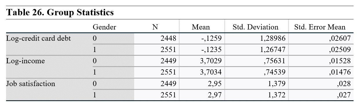
The group statistics show the number of cross section units, mean, standard deviation and standard error mean of each variable for each gender group.
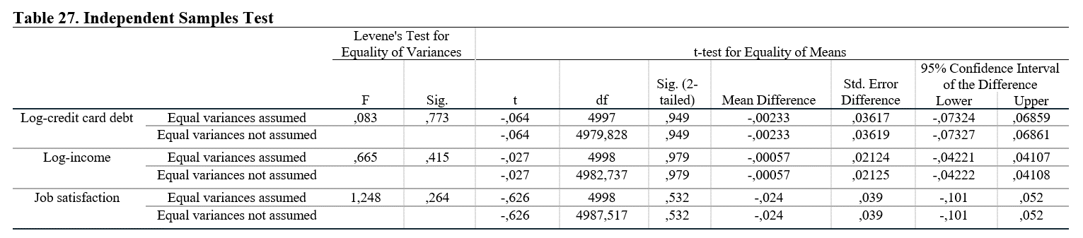
Independent samples test shows our main analysis result. We mentioned about the equal variance assumption that should be hold for the analysis. SPSS allows us to check the results from the independent samples test. For that we need to check Levene’s Test for Equality of Variances results. Sig. (p-value) should be higher than 0.05, so we can assume that the variances are equally distributed. For each variable, the results are higher than 0.05, so we can say that the variances are equally distributed.
For the second step, we need to check T-test for Equality of Means – Sig. (2-tailed) section to see whether there is a difference between two gender groups. In order for us to interpret that there is a statistically significant difference among groups, Sig. (p-value) should be lower than 0.05. As we can see, p-value of none of the variables are lower than 0.05. Therefore, we fail to reject the H0, so we can say that there is no statistically significant difference among gender groups in terms of credit card debt, income and job satisfaction.
If the variances were not equally distributed, we need to check the second line under the T-test for Equality of Means – Sig. (2-tailed) section. In this example both of the lines are equal.
