In the Manova, there are at least two dependent variables in the model. It is possible to have more than one categorical variable (not covariate) in the analysis.
For this example we will use dataset from SPSS samples: customer_dbase.sav
Select customer_dbase.sav.
Click on Analyze section from the top menu.
Find General Linear Model section under Analyze. Then click on Multivariate… button.
Once you clicked you will see the following menu:

We use Commute time in minutes (commutetime) and Log-Credit Card Debt (Increddebt) as dependent variables and level of education (edcat) as categorical independent variable.
As second step, click on the model button:

Use full factorial model and click on Continue button and return to main menu.
Now click on the Post Hoc button and select edcat variable for the post hoc test.
Click on Turkey and Bonferroni tests. You may also click on Tamhane’s and Dunnett’s tests. If the results show that the variances are not equally distributed, you can use the latter tests.
Once you finished, click on Continue button.
Now on the main menu click on Options button.

Select Descriptive Statistics, Estimates of effect size and homogeneity tests and click on continue button.
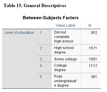
Between-subjects factors table shows how many samples are in each category.
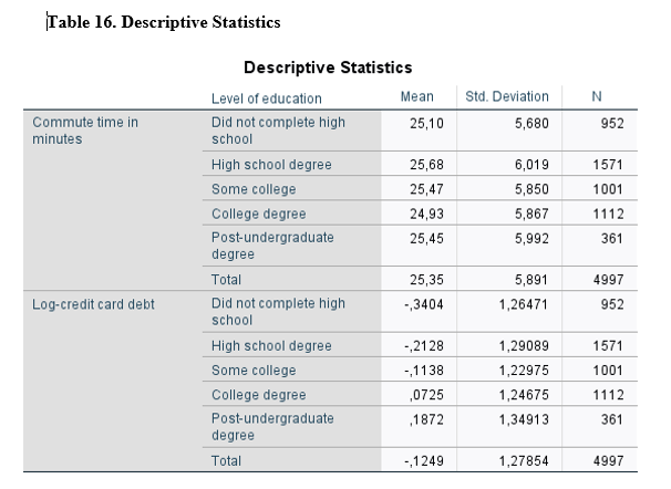
Descriptive statistics table shows how many samples are in each category and their mean and standart deviation.

One of the assumptions of MANOVA is the equality of covariance matrices. As you can see under the result table, the null hypothesis for the test is that covariance matrices of the dependent variables are equal across groups. As results show that the Sig. (p-value) is above 0.05 which means significant. Therefore we accept the null hypothesis and can continue with the analysis.
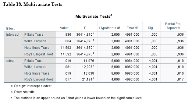
Multivariate tests show that the model is significant since Sig. (p-value) is under 0.05. So we can continue with the analysis.
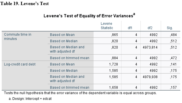
Another assumption of MANOVA is that error variances of the dependent variables are equal across groups. Levene’s test show that Sig. (p-value) of both of the dependent variables are above 0.05. Therefore, we accept the null hypothesis and continue with the analysis.

According to results, there is a significant difference between Commute time of high school and college graduates. Commute time of high school graduates are 75% higher than the college graduates. The main reason of this result can be rationalized as the bargaining power and/or chances of the college graduates are higher than the high school graduates in finding jobs closer where they live.
According to results for Credit Card Debt, there are several significant differences between education categories. In order to keep the example short, we will examine only the people with the College degree. Compared with the people with no high school graduation, high school graduation, some college degree, people with college degree have 41%, 29% and 19% more debt, respectively. There is no significant difference between post-undergraduate degree and college degree. The main reason that the people with college degree have more debt is that these people simply earn more Money, so they have a higher debt. Results show that there is a decrease in percentage when the graduation degree is higher.
