Correlation and regression analyses can be used to examine the relationship between variables while T-test and ANOVA type analyses examine the differences among groups.
Correlation analysis shows the relationship of each variable with each other seperately. Coefficient of the relationship of variable can be either negative or positive. Unlike regression analysis, there may not be a causality between variables.
For this example we will use dataset from SPSS samples: customer_dbase.sav
Select customer_dbase.sav.
Click on Analyze section from the top menu.
Find Correlate section under Analyze. Then click on Bivariate Correlations button.
Once you clicked you will see the following menu:

Normality assumption is important for the correlation analysis. So, if your variables are normally distributed you need to use pearson correlation coefficient, if not use spearman coefficient.
If you assume that there is only one way relationship between variables (i.e. you expect only a positive relationship between variables), you need to choose One-tailed test. If you are not sure or not foresee positive or negative relationship, choose Two-tailed test.
Once you finished, click OK to see the results. For this example, we selected both Pearson and Spearman Coefficients.
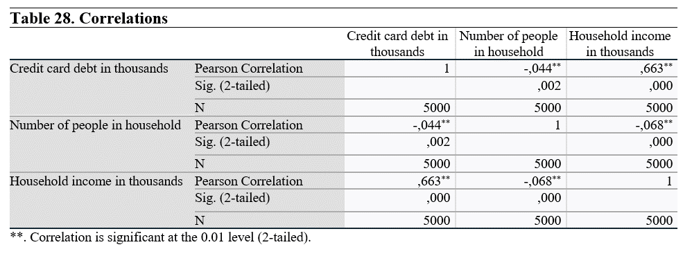
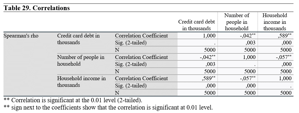
If the sign was *, this would mean that the correlation is significant at 0.05 level.
In both coefficient tests, there are statistically significant relationship between each variable pairs.
Analysis results show that there is a negative correlation between Credit card debt and number of people in the household, and a positive correlation between Credit card debt and household income. We can intrepret that the household generate more income than they spent. That is the reason why there is such relationship.
Regression analysis can be used to examine the effect of the independent variable(s) on the dependent variable. A simple regression function can be illustrated as follows:
Yi = ß0 + ß1x + ɛ
Yi: Dependent variable
ß0: Constant / Intercept
ß1: Slope / Coefficient
x: Independent variable
ɛ: Error term
There can be more than one independent variables in the analysis. Effects of each variable on the dependent variable can be examined with their coefficients. The unobserved effects and variables will be represented by the error term.
For this example we will use dataset from SPSS samples: customer_dbase.sav
Select customer_dbase.sav.
Click on Analyze section from the top menu.
Find Regression section under Analyze. Then click on Linear button.
Once you clicked you will see the following menu:
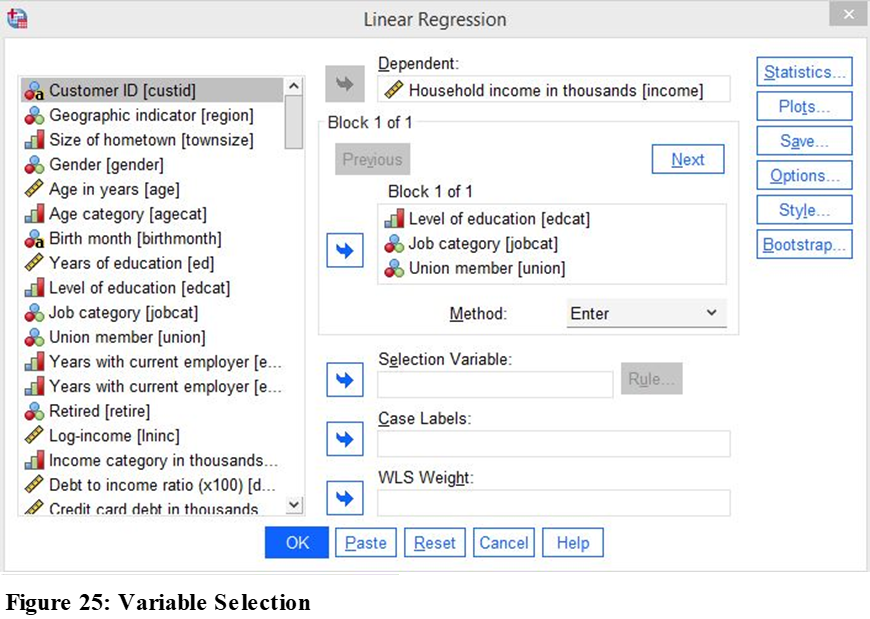
In this example, we will make a multiple regression analysis. We will examine the effects of level of education, job categories and union membership on Household income.
Before we start, I would like to remind you that, your variables should be normally distributed and have equal variance.
Once you selected your variables, click Statistics button on the right:

Select Model fit, descriptives, part and partial correlations, colinearity diagnostics, confidence intervals (as 95%) and click on Continue.
On the main menu click OK to continue to analysis.


In the correlation matrix, it is important to not have a relationship above 0.70. This indicates a strong relationship among variables and yield spurious results. This would indicate multicolinearity problem. In this analysis, we see that there is not a strong relationship between variables. So, we can continue to analysis.
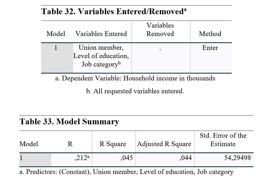
Model summary shows the R values. Since we used a multiple regression model, we need to check Adjusted R Square. This value shows the power of the independent variables to explain the dependent variable. So, from level of education, job category and union membership, only 4.4% of Household income can be explained. This means that there are other contributors that we cannot currently observe and use in the model. If you have more variables, you need to use it in the regression model, otherwise analysis will be effected by unobserved variables.
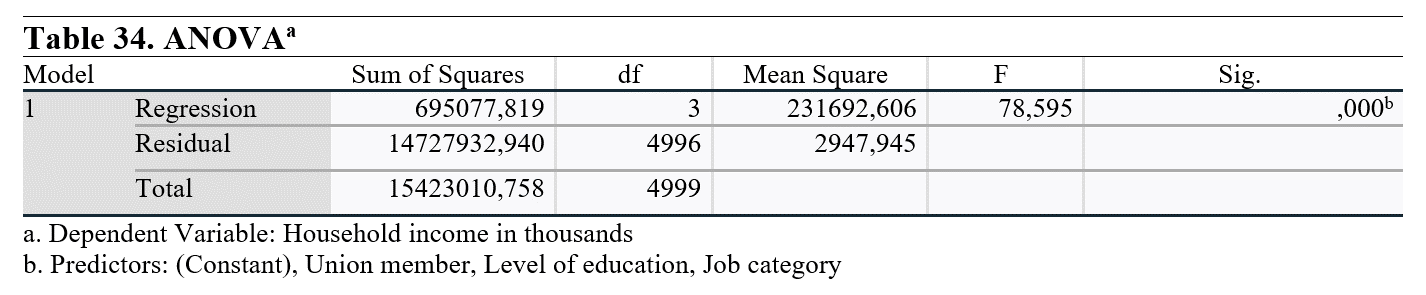
When we checked the Sig. (p-value) of the ANOVA analysis, it can be seen that it is lower than 0.05. This means that at least one variable among independent variables has a statistically significant effect on the dependent variable. For more information about the effect we will examine next analysis.
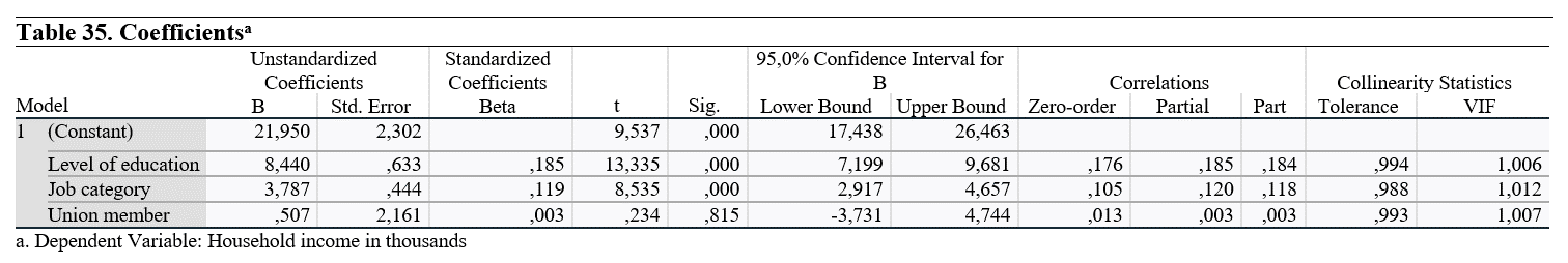
The first thing we need to check in this table is Sig. (p-value). It can be seen that level of education and job category have a significant effect on Household income, on the other hand being a union member has no statistically significant impact on it.
Unstandardized Coefficients show the effect of one unit increase on Household income. So, one level increase in the level of education and job category increase the Household income by 8,440 and 3,787 USD.
Standardized Coefficients show the effect of one unit increase in standard deviation on the standard deviation of Household income.
