Normality is one of the most important assumptions in ANOVA type analysis. So, it is important to check whether each variable in the analysis has a normal distribution.
There are several measures and indicators that you can use to check the normality assumption.
- You can read skewness and kurtosis statistics, values and z-test results.
- You can use Kolmogorov-Smirnov (KS Test) and Shapiro-Wilk Tests (Razali & Wah, 2011).
- You can examine the histogram or any other graphs.


Null hypothesis of the both test are that the data is normally distributed. So, p-values should be higher than 0.05, so we can accept the null hypothesis. However, if samples are more than 300, skewness and kurtosis values should be considered.
Let’s practice the normality test!
Select cross_sell.sav
Click on Analyze button on top menu. Then go to Descriptive Statistics and click on Explore button.
Select following variables and put them on to dependent list:
Special offer purchases [buyoff]
CD purchases [buycd]
Book purchases [buybk]
CD club discount [disccd]
Book club discount [discbk]
Log of CD club discount [lndisccd]
Log of Book club discount [lndiscbk]

After that click on Plots button on the right menu.
Click Histogram under the Descriptive title and also select Normality plots with tests. After that click on Continue button.
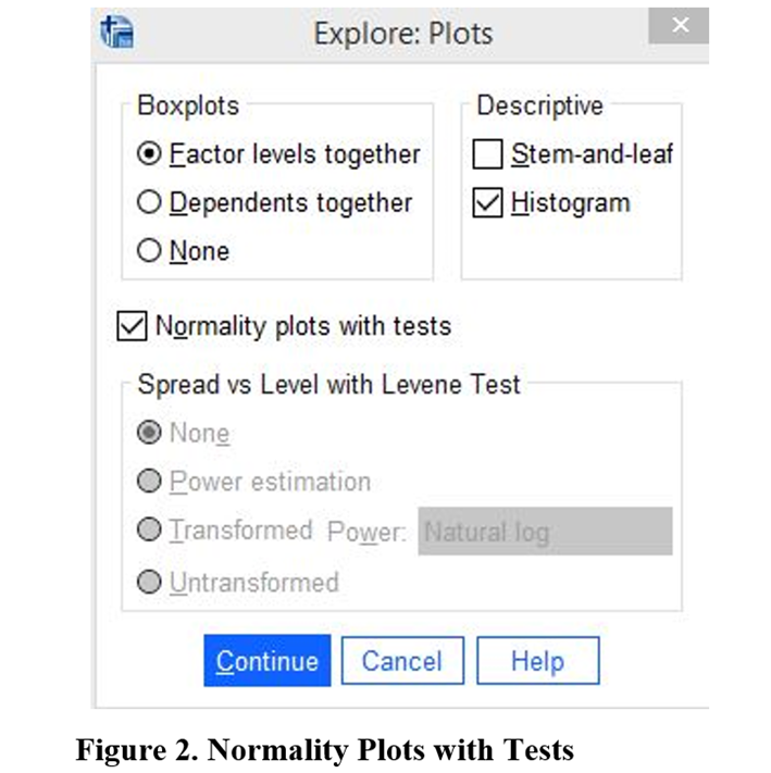
On the main menu click OK to undertake the tests and see the results.
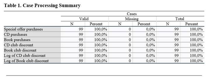

When we examine the descriptive statistics for variables:
Variable: Special offer purchases
Skewness: Statistic: 0.01 Standard Error: 0.243 – Z-Test value: 0.01 / 0.243 = 0.041
Kurtosis Statistic: -0.313 Standard Error: 0.481 – Z-Test value: -0.313 / 0.481 = -0.65
Variable: CD purchases
Skewness: Statistic: 0.237 Standard Error: 0.243 – Z-Test value: 0.237 / 0.243 = 0.975
Kurtosis: Statistic: 0.099 Standard Error: 0.481 – Z-Test value: 0.099 / 0.481 = 0.203
Variable: Book purchases
Skewness: Statistic: -0.194 Standard Error: 0.243 – Z-Test value: -0.194 / 0.243 = -0.798
Kurtosis: Statistic: -0.177 Standard Error: 0.481 – Z-Test value: -0.177 / 0.481 = -0.368
Variable: CD club discount
Skewness: Statistic: 0.615 Standard Error: 0.243 – Z-Test value: 0.615 / 0.243 = 2.53
Kurtosis: Statistic: -0.778 Standard Error: 0.481 – Z-Test value: -0.778 / 0.481 = -1.617
Variable: Book club discount
Skewness: Statistic: 0.682 Standard Error: 0.243 – Z-Test value: 0.682 / 0.243 = 2.81
Kurtosis: Statistic: -0.425 Standard Error: 0.481 – Z-Test value: -0.425 / 0.481 = -0.88
Variable: Log of CD club discount
Skewness: Statistic: -0.332 Standard Error: 0.243 – Z-Test value: -0.332 / 0.243 = -1.37
Kurtosis: Statistic: -1.095 Standard Error: 0.481 – Z-Test value: -1.095 / 0.481 = -2.28
Variable: Log of Book club discount
Skewness: Statistic: -0.407 Standard Error: 0.243 – Z-Test value: -0.407 / 0.243 = -1.674
Kurtosis: Statistic: -0.870 Standard Error: 0.481 – Z-Test value: -0.870 / 0.481 = -1.808
Since the number of N of each variable is 99. It is possible to check the Z-test values in the range of -3.29 and +3.29. Therefore, it can be said that all of the variables are normally distributed.
However, we also need to look for normality test results. Kolmogorov-Smirnov and Shapiro-Wilk tests results show that Special offer purchases, CD purchases and Book purchases are normally distributed since their Sig. (p-value) is bigger than 0.05. For the rest of the variables, we have to reject the null hypothesis. When both of these tests are examined, even though the p-values differ, they yield consistant results.

It is also possible to check the distribution from histogram of the variables. Here is the an example of perfect normal distribution:
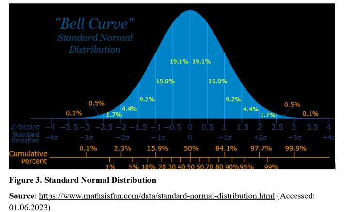

When the histograms are examined, it can be seen that histograms of the first 3 variables which are found to be normally distributed according to normality test results, are more similar with the perfect example of normal distribution. Histograms of the rest of the variables start with a high frequency which decreases gradually and/or by fluctuating.
